A Visual Intuition of Bias and Variance

Bias and variance are two of the most fundamental terms when it comes to statistical modeling, and as such machine learning as well. However, understanding of bias and variance in the machine learning community are somewhat fuzzy, in part because many existing articles on the subject try to produce shorthand analogies (“bias” = “underfit”, “variance” = “overfit”, the bullseye diagrams). While these analogies are fine if you want to quickly describe the performance of a model (“The model has high bias and low variance”), I found that they remove the underlying beauty and concreteness of the bias-variance tradeoff. When it comes to the bullseye diagrams, I found them to leave me even more confused than before (“So bias and variance are essentially accuracy and precision, right?”). I hope that with this article, the reader may find a deeper understanding of bias and variance in statistical modelling. I also hope that they can actually use bias and variance to explain some deeper ideas such as cross-validation.

Many of these ideas are taken from An Introduction to Statistical Learning by Gareth James, Daniela Witten, Trevor Hastie, and Rob Tibshirani.

Statistical Modelling

Bias and variance originate from the field of statistical learning. Statistical learning is a field that tries to put a model on collected data such that (1) they can be predicted or (2) they can be understood.

Example: The very popular Boston housing dataset is a dataset collected by the U.S. Census Service in 1996. It contains multiple variables such as per capita crime rate, number of rooms per dwelling, proportions of non-retail businesses, and price value.

If you want to build a model of the price of houses, you would set other variables to be the predictors of the model and the price of the houses as the response variable. If there are \(p\) different predictors \(X_1, X_2, …, X_p\) and one response variable \(Y\), then we can assume a model of \(Y\) using \(X\) to be:

\begin{align} Y=f(X_1,X_2,…X_p )+\epsilon \end{align}

In this equation, note that besides the function \(f(X)\) that is fixed, there is also another term \(\epsilon\) in the equation. This is the error term. This term is the differences between the modelled value and the actual values and could represent things like noise or random processes. The main takeaway is that \(\epsilon\) is both independent of \(X\) and has a mean value of zero.

Going back to the example, if there is a new house on the listing with all the predictors \(X_{new}\) available and we want to know the price \(Y_{new}\), then we would produce a prediction \(\hat{Y}\) using our model assumption \(\hat{f}\)

\begin{align} \hat{Y}=\hat{f}(X_1,X_2,…X_p ) \end{align}

What is the difference between \(\hat{f}\) and \({f}\)? For once, \({f}\) is the real model that link \(Y\) and \(X\), whereas \(\hat{f}\) is our assumption of what \({f}\) is. Because of this, the real model would always include an independent error value \(\epsilon\), whereas the assumed model would not have this error term because we cannot predict it.

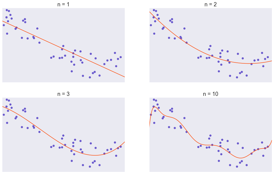
In the real world, if we set out on the task of modelling this data, we likely would not get access to all data points (the collection of all data points is called “population”). Instead, we would only get access to only a selected amount of data points (this is called a “sample”). Here, we have a sample of 50 data points. This will become relevant in our discussion of variance, as multiple sampling of the same population will produce estimation models that are slightly different.

In order to fit a model to this dataset, it is good to start as simple as possible, then moving up in complexity. Here, I will use a polynomial model with \(n^{th}\) power as the highest power, starting with \(n = 1\) (linear regression) then increasing the value of \(n\) all the way up to \(10\). All model are fitted to minimize the mean squared error value.

What is variance?

Now, let’s move onto the main part of this article: developing an understanding of variance and bias. We will talk about variance first because it is simpler to understand. To put simply, not all samples are the same. When sample A and sample B are different, we produce models that look slightly different.

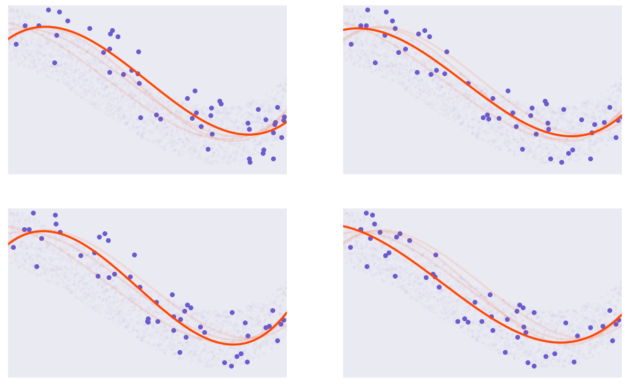
Here we say that we changed the parameters of the model. In the figure above, all models are third order polynomial with \(X^3\) as the highest power. Each models are trained on a slightly different sample of the population.

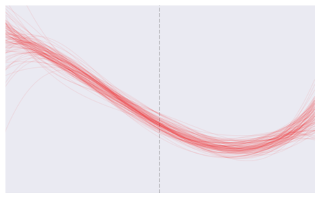
Let’s imagine that we repeat the process 100 times. Here is how they would look.

The goal of our model is to produce predictions. Using the models to predict the \(Y\) value of a new \(X\) yield the following:

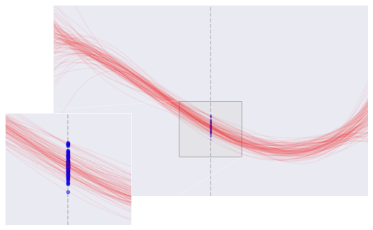
Immediately, we notice that some models produce predictions that varied wildly, but some other models produce predictions that are very consistent. We quantify the consistency by using variance. Statistically, variance of a model prediction is the mean (or expectation) of the squared deviation for all predictions.

Variance refers to the amount by which \(\hat{f}\) would change if we estimated it using a different training data set. Since the training data are used to fit the statistical learning method, different training data sets will result in a different \(\hat{f}\). But ideally the estimate for \(f\) should not vary too much between training sets. However, if a method has high variance then small changes in the training data can result in large changes in \(\hat{f}\). In general, more flexible statistical methods have higher variance.

An Introduction to Statistical Learning

What is bias?

After we produce a variety of predictions, we also want to consider what is the mean, or expected value, of the predictions. This mean value is called the expected value of all predictions, or \(E(\hat{y}_0)\). Bias refers to how much the expected value of all the predictions differs from the actual value.

\begin{align} Bias=E(\hat{y}_0)-y_0 \end{align}

Bias refers to the error that is introduced by approximating a real-life problem, which may be extremely complicated, by a much simpler model. For example, linear regression assumes that there is a linear relationship between \(Y\) and \(X_1, X_2, ..., X_p\). It is unlikely that any real-life problem truly has such a simple linear relationship, and so performing linear regression will undoubtedly result in some bias in the estimate of \(f\).

An Introduction to Statistical Learning

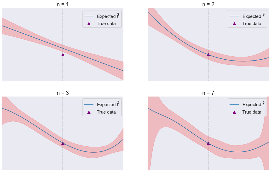
With this figure, I hope you understand how bias and variance are measured and how they can be used to describe models that overfit or underfit.

• In our linear regression model \((n = 1)\), the mean of \(\hat{f}\) is very different from the actual \(Y\) value. The model also have wide range. So we can say that the linear regression model has high bias and high variance.
• In the model using \(n = 7\), the mean of \(\hat{f}\) is very close to the actual \(Y\) value. However, the model have very wide range. We can say that the \(n = 7\) model has low bias but high variance ¹.

• In both the models using \(n = 2\) and \(n = 3\), the variance and the bias are both very small. The goal of statistical modelling is to produce and find models that have both low variance and low bias.

The bias-variance tradeoff

How do we know how “correct” our model is to reality? Well, we did give you a hint in the earlier section. We can calculate the error between the predicted value and the actual value, and then sum them up and take the average. This is, of course, how we arrive at the bias of the predictor. However, doing this will possibly backfire, because if the bias is \(0\), it could mean that the predictor predicts everything correctly (no variance) or that the predictor predicts everything incorrectly but they even out to zero (high variance). Instead, we sum either the absolute value or the square of the error. The square of the error term is more preferred in many cases because it leads to easier implementations in terms of finding a solution. We called it the mean squared error (MSE):

\[\begin{aligned} MSE = \frac{\sum_{n} (\hat{f}_{x_0} - f_{x_0})^2 }{n} \end{aligned}\]

We are summing over all possible \(\hat{f}_{x_0}\), which means all the predictions that different\hat{f}_{x_0} gives depending on the sample we use to train.

If you have taken a statistics course before, you know that this is also called the expected value of the squared error. The expected value has some properties that one can use to decompose the MSE. You should work through the long-form decomposition that Wikipedia and this blog post has derived. In the end, you should get

\[\begin{aligned} MSE &= var(\hat{f}_{x_0}) + (E[\hat{f}_{x_0}] - f_{x_0})^2 + var(\epsilon^2) \\ &= var(\hat{f}_{x_0}) + bias(\hat{f}_{x_0})^2 + var(\epsilon^2) \end{aligned}\]

The \(var(\epsilon^2)\) term is called the irreducible error. It determines the minimum achievable value of the MSE and, in turns, the predictor. As an exercise, can you calculate this value knowing that the error comes from a uniform distribution [-10, 10]?

From this decomposition, it is clear that the MSE is determined by the sum and the bias of the predictors. If we plot the MSE, the variance, and the bias term altogether for models with increasing complexity, we will observe a U-shape value for the MSE. Choosing a correct model requires choosing one that have the appropriate amount of variance and bias.

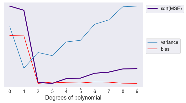
That is the bias – variance tradeoff. In this case, the MSE is lowest at \(n = 3\). We can say that the third-order polynomial best models the actual population.

Question What will happen to the bias and variance of a predictor if I increase the number of training data?

Answer Think intuitively, you will see that by sampling more data points, the resulting predicting model would be more stable. Therefore, the predictor will have a lower variance with increasing training data. The bias, however, will stay the same. This is because the bias simply evens out toward the mean regardless of the number of samples. In reality, if you have too little data points for training, the number of data points would also affect the bias as well because more data points will make the estimator fit better.

Question What will happen to the bias and variance if I add a constant term to my model?

Answer The variance simply measures the spread of the predictions. If I add a constant term, the spread will still stay the same so the variance will stay the same. The bias, on the other hand, will change in the direction of the constant term.

Applications

By now, I hope that you develop an intuition for bias and variance. More specifically, the reason why they are so often used to describe models. However, you might be wondering if they are just words to describe models without actual theoretical nor practical importance. Here, I will guide you through applying bias and variance to cross-validation and classification.

Cross validation

Cross validation is one of the most common methods of assessing your model performance. Usually, to measure model performance, you will split the data into a training set and the validation set, update your model parameters using the training set, and then produce the assessment on the validation set. However, if the original dataset is not large enough, you can repeatedly train the model on different smaller subsets of the original dataset. The final assessment of the model will be a combination of all the assessments using the different validation sets. By looking at the sampling process, you immediately can see how this is related to the variance aspect of the predictor. Our goal is to find the model with the lowest MSE on new test values, so can cross validation do this?

First, let’s consider leave-one-out cross validation (LOOCV). In LOOCV, the testing set only has one sample, and the training set has the rest. The model is trained repeatedly \(n-1\) times, where \(n\) is the number of data points in the dataset. The final assessment is the average of all trainings.

Immediately, you can notice the advantages of LOOCV over simple train-test split without cross-validation. If the existing data sample is good enough, the repeated sampling of the training set is similar to that of repeated sampling of the real population. There is one small caveat, however. When LOOCV is performed, all training samples will have very large overlap. This large overlap can produce high variance of the model.

To reduce the variance, another method of cross-validation called k-fold cross validation can be used instead. In k-fold cross validation, the sample is split into k equal parts. The test set is one part, and the training set is the rest. The model is trained repeatedly k times, each time with a different part for testing. Compared to LOOCV, k-fold validation can produce models with lower variance, but in turn has higher bias.

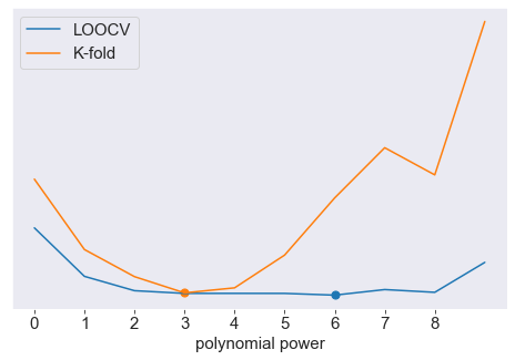
How good is cross-validation is at choosing the best model? Here, we will try to find the best polynomial power using K-fold cross validation \((K = 10)\). LOOCV produce a best value of 6 and K-fold produce a best value of 3. If we don’t want our model to overfit the training sample, we can use the simpler model with \(n = 3\).

Classification

Suppose that you have an interview for a machine learning engineer position. The interviewer asked you:

“What would the effect of increasing the number of K in KNN classifier do to the bias and the variance?”

What would be your answer?

First of all, bias and variance decomposition are derived from mean squared error, which is a term for regression tasks. For KNN, the book Elements of Statistical Learning by Hastie, Tibshirani, and Friedman has a simple decomposition of the error term into a similar sum of bias and variance. All you need to rely on for now is the intuition of bias-variance breakdown from the previous section.

Let’s consider \(K=3\). In this case, any new data will simply be predicted using the closest class. Assuming that this is the behavior of many data points, you would expect that predictions using \(K=3\) will have low bias. However, the decision boundary can vary a lot based on what the class the closest sampled data point would be. Hence, we can say that with small values of \(K\) the predictor tends to have low bias but high variance. Now consider \(K = 10\). In this case, the decision boundaries are much more stable regardless of different training samples. However, if the value of K is too high, then the decision boundaries can become too stable, leading to predictions that are really off. This means that with increasing \(K\), we have models with low variance but have the risk of high bias. The test error rate, which is a summation of both bias and variance terms, will have a characteristic U-shape where the lowest point would correspond to where bias and variance have the best tradeoff.

Here, the boundary using \(K = 1\) is highly varied, while the boundary using \(K = 100\) is stable. We can say that the variance for \(K = 100\) is higher than that for \(K = 1\).Source: James, Witten, Hastie, and Tibshirani

The classification rate (accuracy) in the training and test sets using different value of \(K\). Notice the U-shape in the test set similar to that seen in regression tasks. Source: James, Witten, Hastie, and Tibshirani

Conclusion

I hope that this article will help you understand a little bit more about the intuitions behind bias and variance decomposition. From now you, when thinking about bias and variance of a model, you won’t have to think about analogies such as the dartboard anymore but instead can work out directly from first principles.

If you want to play around with generating the figures, this is the source code. Have fun!

1. Do you notice that the ends of the predictions have very large variance? This is a consequence of Runge’s phenomenon. Please comment if you encountered this before and how you overcame this problem. ↩